James Q. Jacobs - Hopewell Study Resources

Hopewell Study Resources

The materials below are portions of the research product acquired completing a 2002 Hopewell Seminar project, Possible Geodetic Properties and Relationships of Some Monumental Earthworks in the Middle Ohio Valley A Preliminary Inquiry. Subsequently as research continued, many site coordinates were determined with GPS. Some materials are copyrighted by James Q. Jacobs, some are scans of public domain images. Permissions and contact information.

Squier and Davis Survey Maps
Alexandersville Baum Work Blackwater Bourneville Brush Creek Butler County Cedar-Bank Work Dunlaps Works	Great Miami Greene County High Bank Hopeton Hopewell Junction Group Junction Works Liberty Works	Marietta Works Miamisburg Mound Milford Newark Works Newark Gateway Octagon Observatory Paint Creek Works Portsmouth Detail	Portsmouth Works Scioto Valley Seal Works Seip Mound Serpent Mound The Plains, Athens Co. Winchester Worthington

Drawings
Scioto Valley Earthworks Newark and Marietta Relationships Newark Earthworks Outline Marietta Works	High Bank Work, 2 Drawings Liberty Works, 3 Drawings Liberty Works Overlay on Topographic Map Mound City and Hopeton Area Works

Graphics Files
squares circles figure 2 figure 3 figure 5 Figure 6 highbank highbank 2	highbank 3 highbank 4 hopewell hopewell 2 hopewell 3 liberty liberty 2 liberty_highbank_draw liberty_outline	liberty_squier liberty_topo marietta_outline mound_city newark_marietta newark_outline newark_outline2 newark_outline3 Scioto Draw	scioto scioto_area scioto_draw scioto_lat_lon seip seip2 shriver1 shriver2 coordinates

Topographic Maps
Alexander Anderson Baum Bourneville Chillicothe Chillicothe Region Circleville Grave Creek Great Miami Frankfort	Hamilton High Bank Hopeton Hopewell Liberty Little Miami Marietta Massies Creek Miamisburg	Milford Mound City Newark Plains NE Plains NW PlainsSE PlainsSW Pond Creek Portsmouth	Renick Seal Seip Shriver South Portsmouth Turner Detail Turner Winchester WinchesterW
Topographic Map Scans with earthworks and coordinates
Anderson Bourneville Cedar Bank Circleville Frankfort High Bank Topo	High Bank w/coord High Bank Hopeton Liberty Marietta Miamisburg	Milford Moundville Newark Detail Newark Plains Seal Mound	Seip Mound Seip Topo Shriver Tremper Winchester
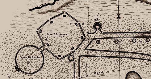
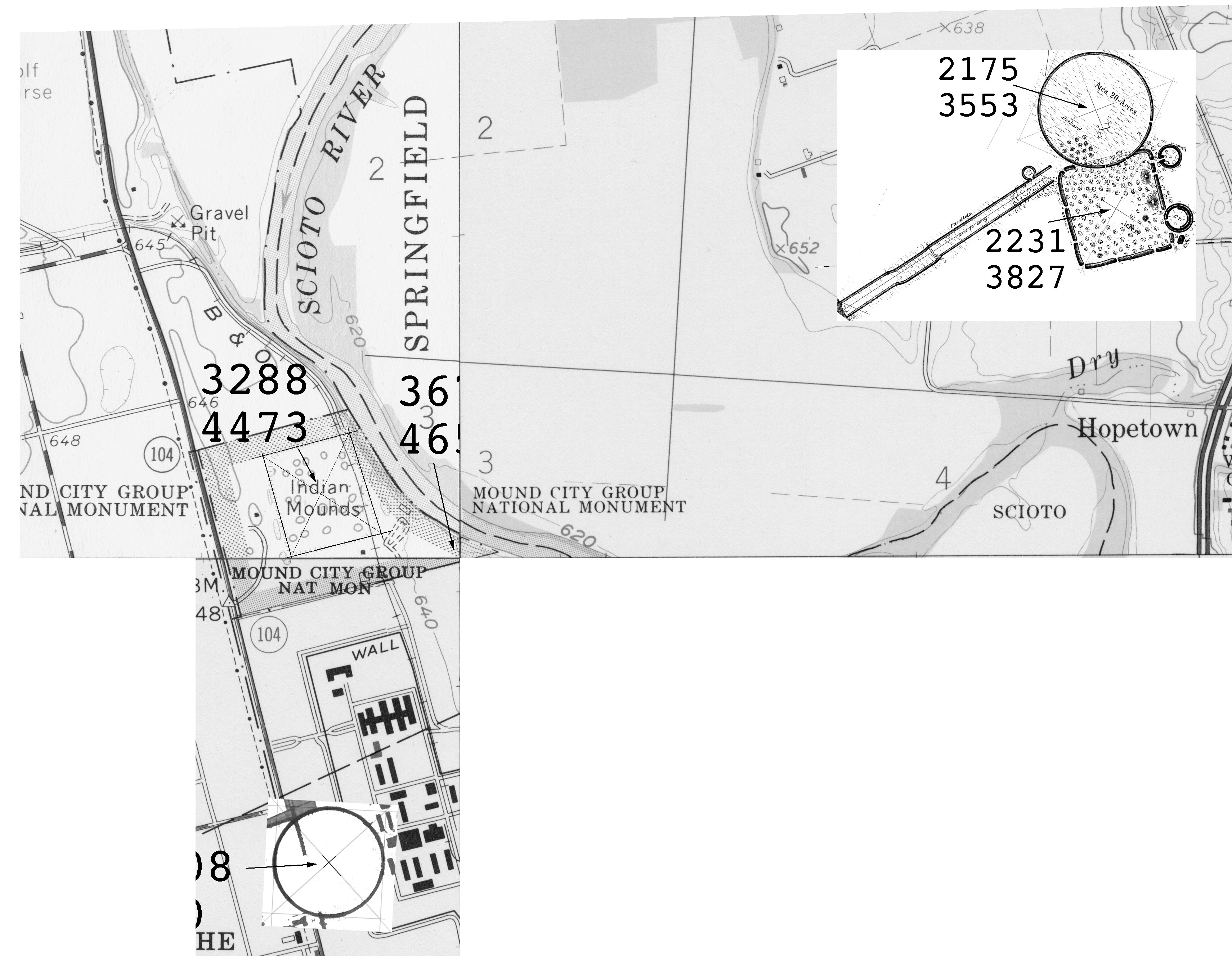
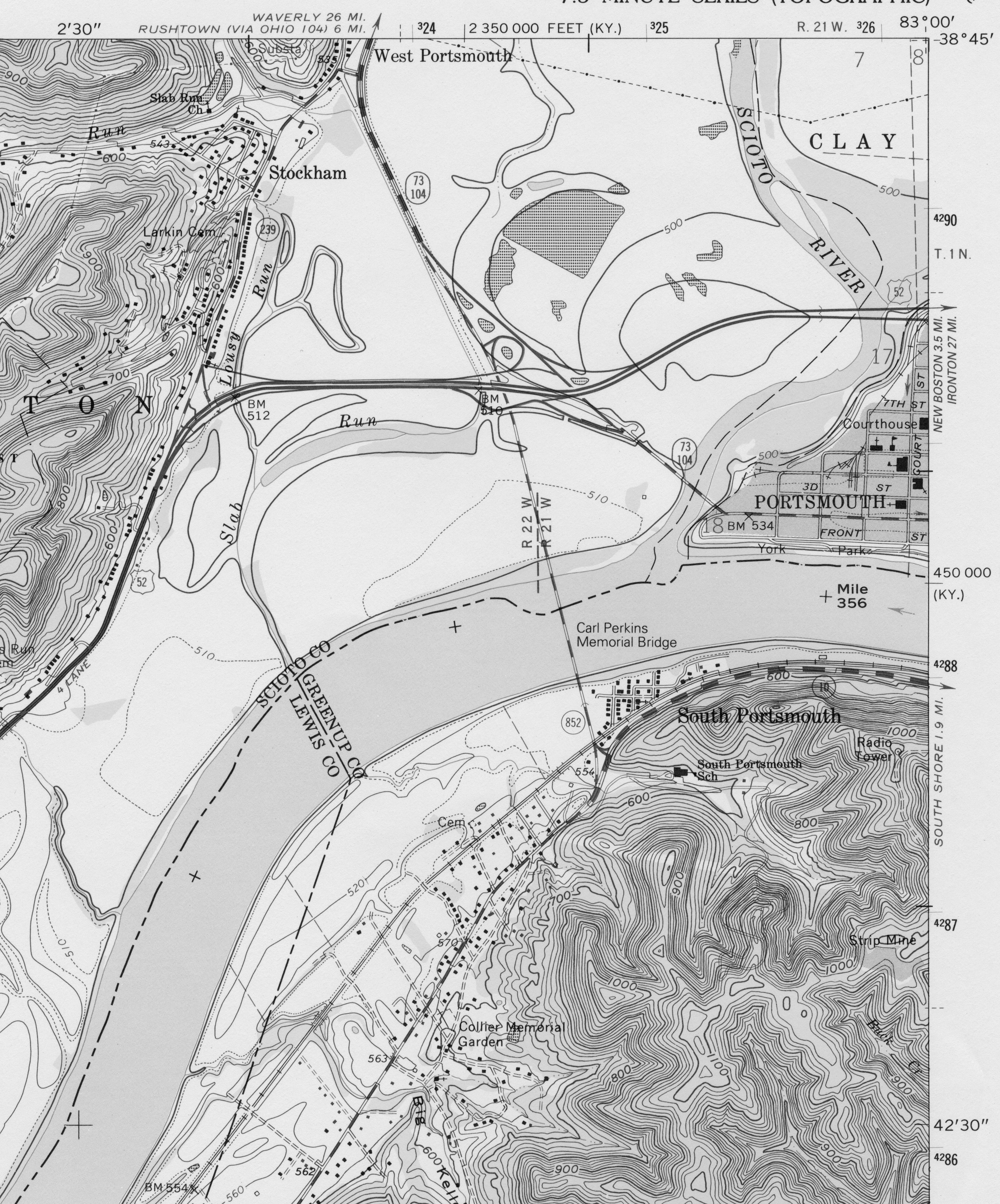
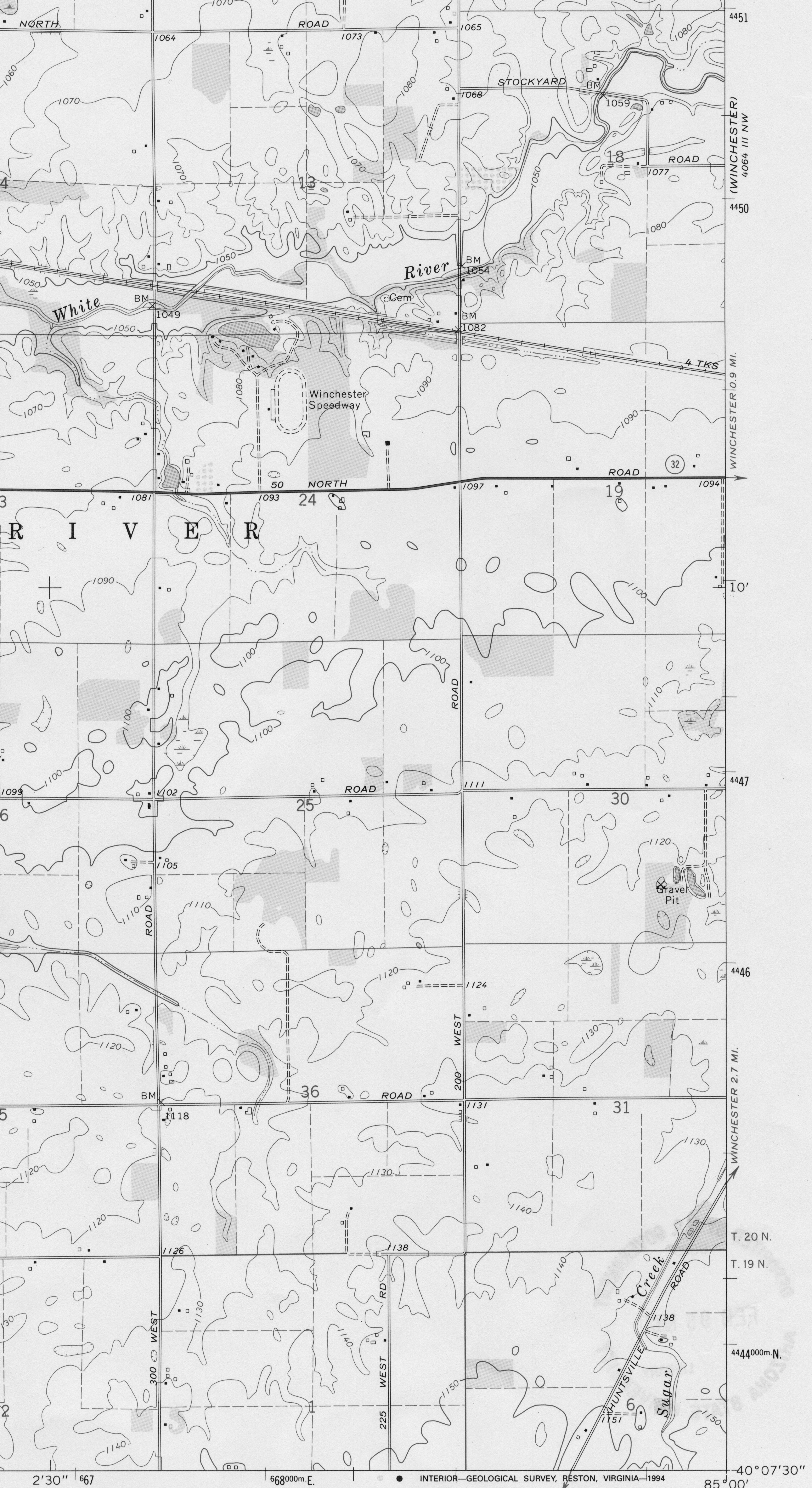
2002 Methods Notes Four coordinates provided by Romain that designate a specific feature of a work were checked against my methods. The mean difference in site location was 224 meters. Coordinates by other authors were ignored. USGS 7.5 minute series topographic maps were scanned at 600 dpi. Squier and Davis illustrations were scanned. High Banks. Placement of the Squier and Davis illustration overlay on the topographic map was determined by Romain’s (2000:23) soil maps and the aerial photography in Hively and Horn (1984:S89). Local roads and railroads were used to place the intersection of the two geometric halves. The 2147.2 feet length was 2246 pixels long. The topo scan was 4566 pixels north-south for 1/24 degree, or 3.3243 feet per pixel given 364,289.413 feet per degree as an Ohio standard. This represents 15,178.73 feet per 1/24 degree north-south, the distance between tick marks on the topo. Liberty. Placement of Squier and Davis’ drawing on the scanned topo was determined using the illustration in Marshall (1987:41), whose determination was made from surveys, aerial photographs and previous surveys. The 1700 foot in diameter circle was scaled to 3.3254 feet per pixel, the scale of the topographic scan. The highway, roadways, railroad, topographic lines and several structures allowed for determination of placement. The Squier and Davis drawing was rotated 92° clockwise and aligned to highway 35, a detail both maps share. Seal. Placement of the scaled Squier and Davis drawing was accomplished using the aerial photography and topographic drawing in Romain (2000:110-111). The Squier and Davis drawing was scaled to the diameter of the circle. The west parallel wall scales to 533 feet., the east to 546. Thomas reports 634 feet. The drawing scales to 363 feet from the square to the ravine along the west parallel wall. Thomas reports 400. Only walls of the square appear in the aerial photograph. The coordinates for the circle are therefore less accurately determined than are the ones for the square. The center of the 1050 foot circle may actually be as much as 100 feet further north than the coordinates on the mapped topo. Hopeton Works. Placement was made using the topographic drawing and the aerial photography in Romain (2000:116-117). Squier and Davis’ map was rotated to align the parallel walls to the mean of Marshall’s survey and to Romain’s survey (57°). Squier’s map was scaled using the diameter of the circle. Placement was oriented by roadways, topo lines, and field boundaries. Hopewell Works. Placement of Squier and Davis was accomplished by placing the square as depicted in Romain (2000:123). Only the square was placed first and then other parts were added. The square size was used to scale the map. Squier and Davis’ north-south line was used to rotate the map 4.61.° Seip Works. Squier and Davis’s map was scaled using a mean of the circle diameter and the square width. Thomas’ azimuth of the square was used to rotate the Squier map. The USGS topo map features the Seip Mound. North-south lines drawn on the Squier map and the USGS map centered on the mound were used to place the Squier map. Frankfort Works. Squier and Davis’ map was rescaled based on three sides of the square valued at 1080 feet and the diameter of the large circle valued at 1480 feet. Placement was made using north-south lines transecting the mound on the topo map and the largest mound in the large circle. Roads and streets were also used in conjunction with the soils map in Romain (2000:23). Newark. The Octagon, Octagon Circle, Octagon Observatory Mound and Newark Circle (Moundbuilders State Memorial) are visible on the topographic map. One pixel lines were used to find the centerpoint of these features. The centerpoint of Newark Square was determined using the survey made by Marshall from the center of Newark Circle 2133 feet east and 2086 feet north at a distance of 2983 feet. Marietta. A scaled drawing based on Squier and Davis was overlayed on the street pattern in Marietta. Illustrations in Romain (2000:132-135) were referenced. Distance from 3rd and Warren to the Conus was used to scale the Squier based drawing. The Quadranau was moved to the center of the park. The large square and small square coordinates are to the centers of the squares. Winchester. The square was placed in the section as illustrated in Squier and Davis. Only the section lines were used as locators. Miamisburg Mound. The center of the top topographic line was used as the point. The feature is clearly drawn on the topographic map. Tremper Mound. The topographic feature is visible on the map. The center of the topographic feature was used. Anderson Square. Aerial photography and a map (Anderson 1980:33-34) were used to locate the center of the feature on the topographic map. Milford Square. Squier and Davis’ drawing was scaled to match the topographic map and pasted in the approximate location as determined from Squier and Davis. The feature did not fit very well to the actual topography, calling into question the accuracy of the Squier and Davis illustration. Nonetheless, the coordinates should fall within the square. Grave Creek Mound. The feature is clearly defined on the topographic map. The center of the feature was used as the coordinate point. Baum Works. This is the only work that was scaled from a digital file, rather than a 600 dpi scan of the topographic map. The resolution of the digital file is 250 dpi. The work was scaled from the Squier and Davis drawing. The outline was rotated to match the survey by Thomas (1894). The work outline was superimposed on the topographic map using the soil map in Romain (2000:23) and the Squier and Davis map as references, with roads, buildings and topography lines as references. The centers of the circles and the square were determined to the nearest pixel.

Soil Map JPEGs
Anderson Baum Cedar Bank	Dunlap Frankfort High Bank	Hopeton Hopewell Liberty	Seip Shriver

Soil Map JPEGs